Figure 5
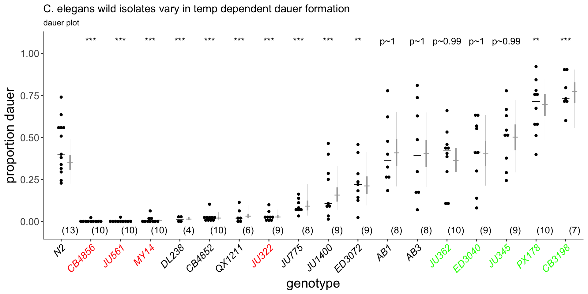
High temperature-induced dauer formation and adult exploratory behaviors do not covary
5A
#knitr::opts_chunk$set(cache=TRUE)
filepath<-file.path(pathname, "extdata","5A_wildHTdata_allbinary.csv")
foods = "OP50"
strains <- c("N2","CB4856","JU561", "MY14","DL238","CB4852","QX1211","JU322","JU775","JU1400","ED3072","AB1","AB3","JU362","ED3040", "JU345","PX178","CB3198")

##"TR403","KR314",CB4507,DR1350 left off due to low n
HT.wildall<-read.csv(filepath, header=TRUE) %>% format_dauer(p.dauer = "exclude")

lm <- HT.wildall %>% dauer_ANOVA()
contrasts<-dunnett_contrasts(lm, ref.index = 1, "genotype")
stan.glmm <- HT.wildall %>% run_dauer_stan
mixed<-stan.glmm %>% getStan_CIs(type = "dauer")

plot.contrasts<-c("",contrasts$prange[1:17])

(p<-plot_CIs(HT.wildall, title='C. elegans wild isolates vary in temp dependent dauer formation', plot.contrasts, ypos = 1.075, type = "dauer", labels = strains)) + theme(
  axis.text.x = element_text(colour =
                               c("black",
                                 rep('red',3),
                                 rep('black',3),
                                 'red',
                                 rep('black',5),
                                 rep('green',5))
                             )
  )
#plot
Figure 5A
Wild isolates vary in high temperature dauer formation. Dauers formed by the indicated C. elegans strains at 27°C. Strains also assayed for exploratory behavior in (B) are in red (weaker Hid phenotype than Bristol N2) and green (similar or stronger Hid phenotype than N2). Each black dot indicates the average number of dauers formed in a single assay. Horizontal black bar indicates median. Light gray thin and thick vertical bars at right indicate Bayesian 95% and 75% credible intervals, respectively. Numbers in parentheses below indicate the number of independent experiments with at least 16 animals each. All shown P-values are with respect to the Bristol N2 strain; ** and *** - different from the Bristol N2 strain at P<0.01 and P<0.001, respectively (ANOVA with Dunnett-type multivariate-t post-hoc adjustment).
library(sjPlot)
sjt.lm(lm, depvar.labels = "number of entries", show.se = TRUE, show.fstat = TRUE)| number of entries | |||||
| B | CI | std. Error | p | ||
| (Intercept) | 0.44 | 0.37 – 0.52 | 0.04 | <.001 | |
| genotype | |||||
| CB4856 | -0.44 | -0.56 – -0.33 | 0.06 | <.001 | |
| JU561 | -0.44 | -0.56 – -0.32 | 0.06 | <.001 | |
| MY14 | -0.43 | -0.55 – -0.32 | 0.06 | <.001 | |
| DL238 | -0.43 | -0.59 – -0.27 | 0.08 | <.001 | |
| CB4852 | -0.42 | -0.54 – -0.30 | 0.06 | <.001 | |
| QX1211 | -0.41 | -0.54 – -0.27 | 0.07 | <.001 | |
| JU322 | -0.41 | -0.53 – -0.29 | 0.06 | <.001 | |
| JU775 | -0.35 | -0.48 – -0.23 | 0.06 | <.001 | |
| JU1400 | -0.25 | -0.37 – -0.13 | 0.06 | <.001 | |
| ED3072 | -0.21 | -0.33 – -0.09 | 0.06 | <.001 | |
| AB1 | -0.03 | -0.15 – 0.09 | 0.06 | .640 | |
| AB3 | -0.02 | -0.15 – 0.10 | 0.06 | .730 | |
| JU362 | -0.06 | -0.18 – 0.05 | 0.06 | .299 | |
| ED3040 | -0.03 | -0.15 – 0.09 | 0.06 | .625 | |
| JU345 | 0.06 | -0.06 – 0.18 | 0.06 | .301 | |
| PX178 | 0.24 | 0.12 – 0.35 | 0.06 | <.001 | |
| CB3198 | 0.32 | 0.19 – 0.45 | 0.07 | <.001 | |
| Observations | 159 | ||||
| R2 / adj. R2 | .769 / .741 | ||||
| F-statistics | 27.580*** | ||||
knitr::kable(contrasts, caption = "pairwise comparisons (ANOVA)")| contrast | estimate | SE | df | t.ratio | p.value | prange |
|---|---|---|---|---|---|---|
| CB4856 - N2 | -0.4409536 | 0.0585877 | 141 | -7.5263826 | 0.0000000 | *** |
| JU561 - N2 | -0.4406758 | 0.0585877 | 141 | -7.5216414 | 0.0000000 | *** |
| MY14 - N2 | -0.4334073 | 0.0585877 | 141 | -7.3975793 | 0.0000000 | *** |
| DL238 - N2 | -0.4296227 | 0.0796411 | 141 | -5.3944862 | 0.0000053 | *** |
| CB4852 - N2 | -0.4198412 | 0.0585877 | 141 | -7.1660268 | 0.0000000 | *** |
| QX1211 - N2 | -0.4074181 | 0.0687454 | 141 | -5.9264755 | 0.0000004 | *** |
| JU322 - N2 | -0.4127995 | 0.0603994 | 141 | -6.8344955 | 0.0000000 | *** |
| JU775 - N2 | -0.3513550 | 0.0625903 | 141 | -5.6135662 | 0.0000019 | *** |
| JU1400 - N2 | -0.2507300 | 0.0603994 | 141 | -4.1511991 | 0.0008539 | *** |
| ED3072 - N2 | -0.2122871 | 0.0603994 | 141 | -3.5147202 | 0.0088605 | ** |
| AB1 - N2 | -0.0293200 | 0.0625903 | 141 | -0.4684431 | 0.9999994 | p~1 |
| AB3 - N2 | -0.0216323 | 0.0625903 | 141 | -0.3456173 | 1.0000000 | p~1 |
| JU362 - N2 | -0.0610929 | 0.0585877 | 141 | -1.0427596 | 0.9856297 | p~0.99 |
| ED3040 - N2 | -0.0296249 | 0.0603994 | 141 | -0.4904834 | 0.9999988 | p~1 |
| JU345 - N2 | 0.0626901 | 0.0603994 | 141 | 1.0379262 | 0.9862469 | p~0.99 |
| PX178 - N2 | 0.2362373 | 0.0585877 | 141 | 4.0321992 | 0.0014339 | ** |
| CB3198 - N2 | 0.3230826 | 0.0652993 | 141 | 4.9477178 | 0.0000384 | *** |
S3
filepath<-file.path(pathname, "extdata","S3A_C3_sumstats.csv")
C327<-read.csv(filepath, header=TRUE)

(p<-dauergut::plot_regression_se(C327, "mean.C3", "mean.HT","SEM.C3", "SEM.HT"))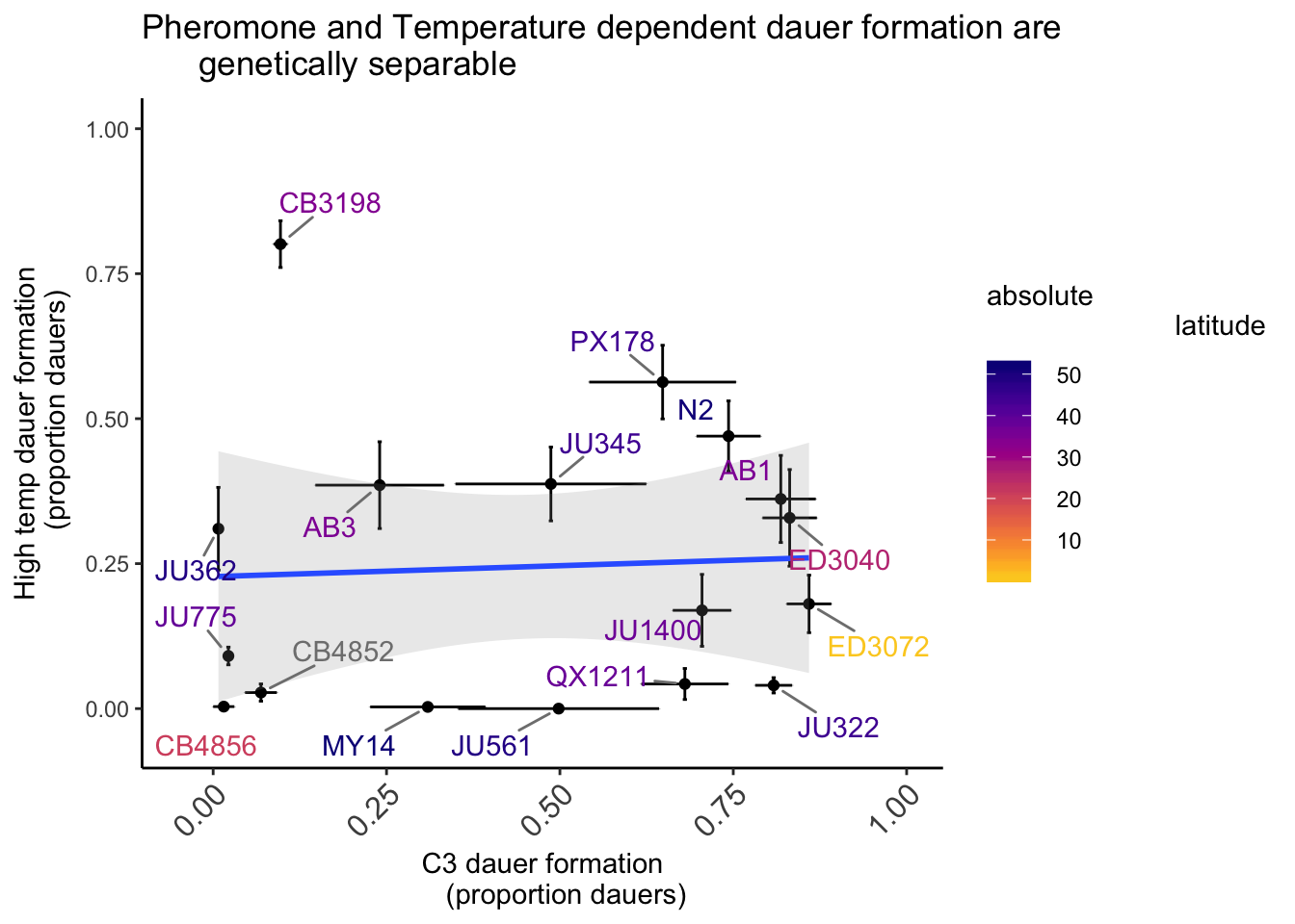
Figure S3
Shown are the proportion of dauers formed at 27°C and in the presence of 6 μm ascr#5 pheromone by C. elegans strains isolated from different latitudes. Assays were performed on live OP50. For ascr#5 data (A-axis), each data point is the average of at least 3 independent assays of at least 23 animals each. 27ºC data is repeated from Figure 6A. Error bars are the SEM. Line and shaded region indicate linear regression fit using mean dauer formation values for each strain.
5B
strains <- c("N2","CB4856", "JU561", "MY14", "JU322", "JU362","ED3040", "JU345", "PX178", "CB3198")

wild.roam<-read.csv(file.path(pathname, "extdata","5B_6F_roam_wild_isolates.csv")) %>%
  dplyr::filter(genotype %in% strains) %>%
  mutate(genotype = factor(genotype, levels = strains),
         strainDate = interaction(genotype, date, drop=TRUE),
         plateID = interaction(strainDate,plate, drop=TRUE),
         total.boxes = 186)

lm <- lm(n_entries ~ genotype, data = wild.roam)

wild.roam %<>% dauergut::flag_outliers(df = ., lin.mod = lm, threshold = 4, noplot=TRUE)

stan.glmm <- stan_glmer(data = wild.roam[wild.roam$outlier.status == FALSE,],
                        formula = n_entries ~ genotype + (1|date/plateID), family = "poisson",
                        iter = 4000, adapt_delta = 0.99)

lm <- update(lm, data = wild.roam[wild.roam$outlier.status == FALSE,])
glmm.nest <- glmer(data=wild.roam, n_entries ~ genotype + (1|date/plateID), family="poisson")

contrasts<-dauergut::tukey_contrasts(glmm.nest, "genotype")
mixed<-stan.glmm %>% getStan_CIs(type = "roam")
plot.contrasts<-c("",contrasts$prange[1:9])


(p<-plot_CIs(wild.roam, title='Foraging behavior is not correlated with Hid phenotypes', plot.contrasts=plot.contrasts, ypos = 800, offset = 50, type = "grid", labels = strains)) + theme(
  axis.text.x = element_text(colour = c("black", rep('red',4), rep('green',5)))
)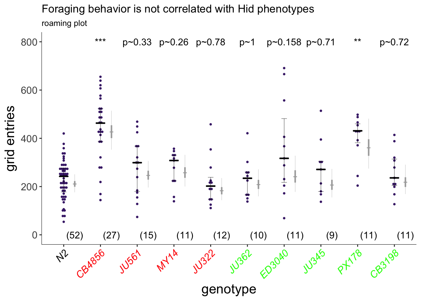
Figure 5B
Exploratory behavior of indicated strains. Strains in red and green exhibit weaker or similar/stronger Hid phenotypes than N2, respectively (A). Each purple dot is data from a single animal. Median is indicated by a black horizontal line; error bars are quartiles. Light gray thin and thick vertical bars at right indicate Bayesian 95% and 75% credible intervals, respectively. Numbers in parentheses below indicate the total number of animals examined in at least 3 independent assay days. P-values shown are with respect to N2; *** - different from N2 at P<0.001 (ANOVA with Dunnett-type multivariate-t post-hoc adjustment).
library(sjPlot)
sjt.glmer(glmm.nest, depvar.labels = "number of entries", show.se = TRUE)| number of entries | |||||
| IRR | CI | std. Error | p | ||
| Fixed Parts | |||||
| (Intercept) | 210.34 | 184.15 – 240.25 | 14.27 | <.001 | |
| genotype (CB4856) | 1.97 | 1.63 – 2.38 | 0.19 | <.001 | |
| genotype (JU561) | 1.18 | 0.94 – 1.50 | 0.14 | .160 | |
| genotype (MY14) | 1.24 | 0.95 – 1.63 | 0.17 | .109 | |
| genotype (JU322) | 0.95 | 0.73 – 1.23 | 0.13 | .677 | |
| genotype (JU362) | 1.00 | 0.75 – 1.33 | 0.15 | .997 | |
| genotype (ED3040) | 1.33 | 0.99 – 1.77 | 0.20 | .056 | |
| genotype (JU345) | 1.11 | 0.81 – 1.51 | 0.17 | .526 | |
| genotype (PX178) | 1.67 | 1.25 – 2.24 | 0.25 | <.001 | |
| genotype (CB3198) | 1.08 | 0.81 – 1.44 | 0.16 | .596 | |
| Random Parts | |||||
| τ00, plateID:date | 0.155 | ||||
| τ00, date | 0.013 | ||||
| NplateID:date | 169 | ||||
| Ndate | 9 | ||||
| ICCplateID:date | 0.132 | ||||
| ICCdate | 0.011 | ||||
| Observations | 169 | ||||
| Deviance | 6.846 | ||||
knitr::kable(drop1(glmm.nest, test = "Chisq"), caption = "Wald chi square test")| Df | AIC | LRT | Pr(Chi) | |
|---|---|---|---|---|
| NA | 2087.414 | NA | NA | |
| genotype | 9 | 2124.091 | 54.67739 | 0 |
knitr::kable(contrasts, caption = "pairwise comparisons (GLMM)")| contrast | rate.ratio | SE | df | z.ratio | p.value | prange |
|---|---|---|---|---|---|---|
| N2 - CB4856 | 0.5083058 | 0.0495027 | NA | -6.9482277 | 0.0000000 | *** |
| N2 - JU561 | 0.8442069 | 0.1017525 | NA | -1.4051055 | 0.3272521 | p~0.33 |
| N2 - MY14 | 0.8036547 | 0.1095922 | NA | -1.6029182 | 0.2550498 | p~0.26 |
| N2 - JU322 | 1.0568465 | 0.1401219 | NA | 0.4170120 | 0.7807726 | p~0.78 |
| N2 - JU362 | 1.0005047 | 0.1453279 | NA | 0.0034738 | 0.9972283 | p~1 |
| N2 - ED3040 | 0.7540483 | 0.1114761 | NA | -1.9095308 | 0.1581648 | p~0.158 |
| N2 - JU345 | 0.9048790 | 0.1426752 | NA | -0.6339315 | 0.7130674 | p~0.71 |
| N2 - PX178 | 0.5978794 | 0.0892449 | NA | -3.4458981 | 0.0042687 | ** |
| N2 - CB3198 | 0.9245871 | 0.1366262 | NA | -0.5306087 | 0.7244878 | p~0.72 |
| CB4856 - JU561 | 1.6608247 | 0.2189335 | NA | 3.8484756 | 0.0013371 | ** |
| CB4856 - MY14 | 1.5810456 | 0.2284924 | NA | 3.1697135 | 0.0076295 | ** |
| CB4856 - JU322 | 2.0791549 | 0.2995088 | NA | 5.0811910 | 0.0000084 | *** |
| CB4856 - JU362 | 1.9683125 | 0.3112340 | NA | 4.2826142 | 0.0002771 | *** |
| CB4856 - ED3040 | 1.4834540 | 0.2390780 | NA | 2.4470438 | 0.0540125 | p~0.054 |
| CB4856 - JU345 | 1.7801862 | 0.3024871 | NA | 3.3940796 | 0.0044267 | ** |
| CB4856 - PX178 | 1.1762199 | 0.1911839 | NA | 0.9985532 | 0.5110894 | p~0.51 |
| CB4856 - CB3198 | 1.8189583 | 0.2941548 | NA | 3.6994709 | 0.0019444 | ** |
| JU561 - MY14 | 0.9519642 | 0.1520429 | NA | -0.3082233 | 0.7931642 | p~0.79 |
| JU561 - JU322 | 1.2518810 | 0.1944984 | NA | 1.4459328 | 0.3175630 | p~0.32 |
| JU561 - JU362 | 1.1851416 | 0.1988868 | NA | 1.0121881 | 0.5110894 | p~0.51 |
| JU561 - ED3040 | 0.8932032 | 0.1512789 | NA | -0.6668437 | 0.7099762 | p~0.71 |
| JU561 - JU345 | 1.0718688 | 0.1901897 | NA | 0.3911443 | 0.7826519 | p~0.78 |
| JU561 - PX178 | 0.7082143 | 0.1210507 | NA | -2.0184930 | 0.1399498 | p~0.14 |
| JU561 - CB3198 | 1.0952139 | 0.1859918 | NA | 0.5355577 | 0.7244878 | p~0.72 |
| MY14 - JU322 | 1.3150505 | 0.2231575 | NA | 1.6139257 | 0.2550498 | p~0.26 |
| MY14 - JU362 | 1.2449435 | 0.2279188 | NA | 1.1967196 | 0.4186275 | p~0.42 |
| MY14 - ED3040 | 0.9382740 | 0.1741248 | NA | -0.3433199 | 0.7931642 | p~0.79 |
| MY14 - JU345 | 1.1259549 | 0.2173040 | NA | 0.6146861 | 0.7130674 | p~0.71 |
| MY14 - PX178 | 0.7439506 | 0.1389804 | NA | -1.5832897 | 0.2550498 | p~0.26 |
| MY14 - CB3198 | 1.1504780 | 0.2146873 | NA | 0.7511911 | 0.6569095 | p~0.66 |
| JU322 - JU362 | 0.9466887 | 0.1655377 | NA | -0.3133080 | 0.7931642 | p~0.79 |
| JU322 - ED3040 | 0.7134889 | 0.1261605 | NA | -1.9091993 | 0.1581648 | p~0.158 |
| JU322 - JU345 | 0.8562066 | 0.1580227 | NA | -0.8411485 | 0.6211004 | p~0.62 |
| JU322 - PX178 | 0.5657202 | 0.1007625 | NA | -3.1982696 | 0.0076295 | ** |
| JU322 - CB3198 | 0.8748546 | 0.1555674 | NA | -0.7518664 | 0.6569095 | p~0.66 |
| JU362 - ED3040 | 0.7536679 | 0.1342568 | NA | -1.5875535 | 0.2550498 | p~0.26 |
| JU362 - JU345 | 0.9044225 | 0.1694381 | NA | -0.5362255 | 0.7244878 | p~0.72 |
| JU362 - PX178 | 0.5975778 | 0.1065366 | NA | -2.8879775 | 0.0174477 | p~0.017 |
| JU362 - CB3198 | 0.9241207 | 0.1647885 | NA | -0.4425357 | 0.7793309 | p~0.78 |
| ED3040 - JU345 | 1.2000279 | 0.2151714 | NA | 1.0169515 | 0.5110894 | p~0.51 |
| ED3040 - PX178 | 0.7928927 | 0.1345797 | NA | -1.3672532 | 0.3356334 | p~0.34 |
| ED3040 - CB3198 | 1.2261643 | 0.2094249 | NA | 1.1937626 | 0.4186275 | p~0.42 |
| JU345 - PX178 | 0.6607286 | 0.1186767 | NA | -2.3072252 | 0.0728386 | p~0.073 |
| JU345 - CB3198 | 1.0217798 | 0.1842493 | NA | 0.1194865 | 0.9254556 | p~0.93 |
| PX178 - CB3198 | 1.5464441 | 0.2648507 | NA | 2.5455278 | 0.0446370 | p~0.045 |