Intestinal mTORC2 regulates sensory neuron state
2A
strains<-c("N2","mg360","ft7","ft7_ges1resc", "ft7_ifb2resc", "ft7_gpa4resc")
dates<-c("10_22_16", "11_9_16", "11_23_16", "12_16_17", "12_20_17") #dropped "12_6_16" due to missingness
d7GFP<-read.csv(file.path(pathname,"extdata","2A_3A_daf7GFP.csv")) %>%
  filter(mean!=4095 & genotype %in% strains & date %in% dates & temp == "27" & food == "OP50") %>%
  mutate(genotype = factor(genotype, levels=strains),
         ID = as.character(ID),
         date = factor(date, levels = dates),
         dataset = case_when(date %in% dates[1:3] ~ "1",
                             date %in% dates[4:5] ~ "2")) %>%
  separate(ID, c("ID.A", "ID.B"), sep = ":", extra = "drop") %>%
  mutate(genoID = paste(date, genotype, ID.A, sep = ":"), cell.norm = mean) %>%
  filter(note == "")

df <- d7GFP %>%
  group_by(date, genotype, genoID, dataset) %>%
  summarise(cell.norm = mean(cell.norm)) # take mean of each worm

#normalize to mean ft7 each day
day.means <- df %>%
  filter(genotype == "ft7") %>%
  group_by(date) %>%
  summarise(mean_ft7 = mean(cell.norm)) %>% data.frame()

df %<>% mutate(cell.norm = case_when(
  date == dates[1] ~ cell.norm,
  date == dates[2] ~ (cell.norm * day.means[1,2]) / day.means[2,2],
  date == dates[3] ~ (cell.norm * day.means[1,2]) / day.means[3,2],
  date == dates[4] ~ (cell.norm * day.means[1,2]) / day.means[4,2],
  date == dates[5] ~ (cell.norm * day.means[1,2]) / day.means[5,2]
)) %>% data.frame()


log.tran<-lsmeans::make.tran(type="genlog", param = c(0,10))
linmod <- with(log.tran, lm(linkfun(cell.norm) ~ genotype, data = df))
df <- flag_outliers(linmod, df = df, threshold = 4, noplot = TRUE)


# ### Linear models ###
linmod <- with(log.tran, lm(linkfun(cell.norm) ~ genotype, data = df[df$outlier.status == FALSE,]))


stanlmer <- with(log.tran, rstanarm::stan_lmer(linkfun(cell.norm) ~ genotype + (1|date) + (1|genotype:date),
                                               data = df[df$outlier.status == FALSE,],
                                               chains = 3,
                                               cores =4,
                                               seed = 2000,
                                               iter=6000,
                                               control = list(adapt_delta=0.99)))

#refit stanlmer using ft7 as reference to get credible interval for ifb-2 rescue:
df2 <- df %>% mutate(genotype = factor(genotype, levels = c(strains[3],strains[1:2],strains[4:6])))
stanlmer2 <- with(log.tran, rstanarm::stan_lmer(linkfun(cell.norm) ~ genotype + (1|date) + (1|genotype:date),
                                               data = df2[df2$outlier.status == FALSE,],
                                               chains = 3,
                                               cores =4,
                                               seed = 2000,
                                               iter=6000,
                                               control = list(adapt_delta=0.99)))
#
stanlmer3 <- with(log.tran, rstanarm::stan_lmer(linkfun(cell.norm) ~ genotype + (1 + genotype|date),
                                               data = df2[df2$outlier.status == FALSE,],
                                               chains = 3,
                                               cores =4,
                                               seed = 2000,
                                               iter=6000,
                                               control = list(adapt_delta=0.99)))

PI_ifb2 <- rstanarm::posterior_interval(stanlmer2, pars = "(Intercept)", regex_pars = "ifb", prob = 0.90)
p2 <- plot(stanlmer3, pars = "beta") #, regex_pars = "genotype")

contrasts <- tukey_contrasts(linmod, factor = "genotype")
plot.contrasts <- c("",contrasts$prange[1:5])
plot.contrasts.2 <- c("","","",contrasts$prange[10:12])

mixed <- stanlmer %>% dauergut::getStan_CIs(type = "log", base = 10)

labels <- c("WT","rict-1(mg360)",
            "rict-1(ft7)",
            "rict-1(ft7); +ges1p::rict-1",
            "rict-1(ft7); +ifb2p::rict-1",
            "rict-1(ft7); +gpa4p::rict-1") %>% stringr::str_wrap(width = 10)

p <- df[df$outlier.status == FALSE,] %>%
  dauergut::plot_CIs(df = .,
                     plot.contrasts = plot.contrasts,
                     plot.contrasts.2 = plot.contrasts.2,
                     type = "GFP",
                     title = "",
                     labels = labels,
                     ypos = 6000,
                     offset = 500)

img.path <- file.path(pathname,"figures","2A_daf7GFP.png")
include_graphics(img.path)
p
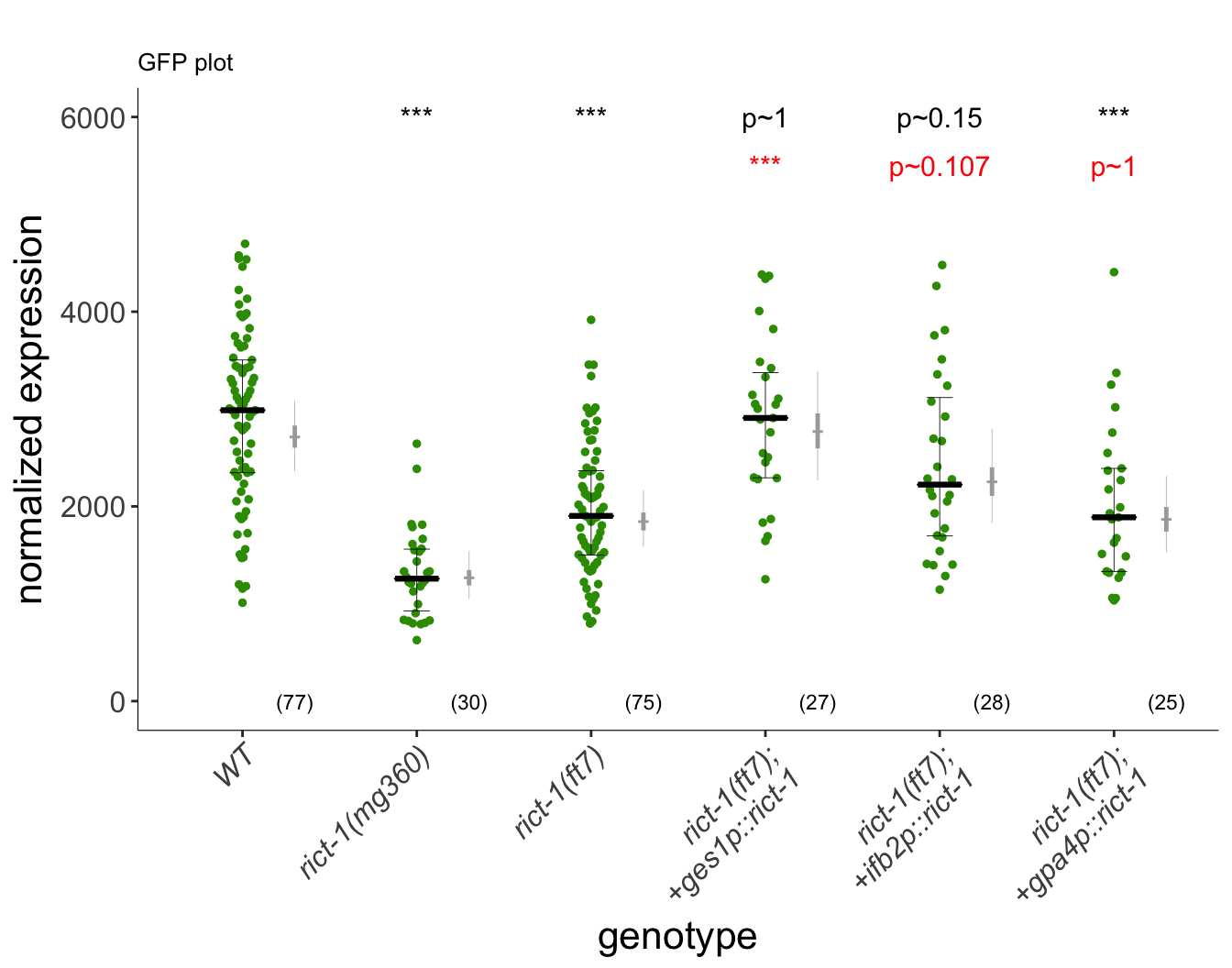
Figure 2A
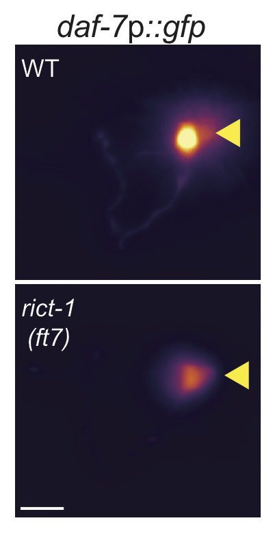
Intesinal rict-1 regulates daf7GFP levels in ASI neurons. Daf-7::GFP fluorescence quantification shows decreased expression in rict-1 mutants. Intestinal expression of rict-1 using the intestinal ges-1 promoter rescues daf-7::GFP expression. (Left) Representative images of daf-7p::gfp expression in one of the bilateral ASI neurons in animals of the indicated genotypes. Yellow filled and open arrowheads indicate ASI and ASJ soma, respectively. Anterior is at left. Scale bar: 5 μm. (Right) Quantification of daf-7p::gfp expression in ASI (A) and daf-28p::gfp expression in ASI and ASJ (D). Each dot is the mean fluorescence intensity in a single animal (2 neurons per animal); numbers in parentheses below indicate the number of animals examined in 3 independent experiments. Horizontal thick bar indicates median. Error bars are quartiles. Light gray thin and thick vertical bars at right indicate Bayesian 95% and 75% credible intervals, respectively. ** and *** - different from wild-type at P<0.01 and P<0.001, respectively; *** - different from rict-1(ft7) at P<0.001 (ANOVA with Dunnett-type multivariate-t post-hoc adjustment). P-values of differences in means relative to wild-type and corresponding mutant animals are indicated in black and red, respectively.
library(sjPlot)
sjt.lm(linmod, depvar.labels = "log(mean GFP intensity) (AU)", show.se = TRUE, show.fstat = TRUE)
|
|
|
log(mean GFP intensity) (AU)
|
|
|
|
B
|
CI
|
std. Error
|
p
|
|
(Intercept)
|
|
3.44
|
3.41 – 3.48
|
0.02
|
<.001
|
|
genotype
|
|
mg360
|
|
-0.34
|
-0.41 – -0.28
|
0.03
|
<.001
|
|
ft7
|
|
-0.17
|
-0.22 – -0.12
|
0.03
|
<.001
|
|
ft7_ges1resc
|
|
-0.00
|
-0.07 – 0.07
|
0.03
|
.966
|
|
ft7_ifb2resc
|
|
-0.08
|
-0.15 – -0.02
|
0.03
|
.017
|
|
ft7_gpa4resc
|
|
-0.16
|
-0.23 – -0.09
|
0.04
|
<.001
|
|
Observations
|
|
262
|
|
R2 / adj. R2
|
|
.345 / .332
|
|
F-statistics
|
|
26.954***
|
knitr::kable(contrasts, caption="Pairwise comparisons from ANOVA (Dunnett)")
Pairwise comparisons from ANOVA (Dunnett)
| N2 - mg360 |
0.3444142 |
0.0335336 |
256 |
10.2707328 |
0.0000000 |
*** |
| N2 - ft7 |
0.1713309 |
0.0252778 |
256 |
6.7779166 |
0.0000000 |
*** |
| N2 - ft7_ges1resc |
0.0014747 |
0.0348484 |
256 |
0.0423173 |
1.0000000 |
p~1 |
| N2 - ft7_ifb2resc |
0.0829684 |
0.0343846 |
256 |
2.4129517 |
0.1500482 |
p~0.15 |
| N2 - ft7_gpa4resc |
0.1642824 |
0.0358656 |
256 |
4.5804970 |
0.0001159 |
*** |
| mg360 - ft7 |
-0.1730833 |
0.0336587 |
256 |
-5.1423072 |
0.0000072 |
*** |
| mg360 - ft7_ges1resc |
-0.3429395 |
0.0413322 |
256 |
-8.2971489 |
0.0000000 |
*** |
| mg360 - ft7_ifb2resc |
-0.2614458 |
0.0409419 |
256 |
-6.3857752 |
0.0000000 |
*** |
| mg360 - ft7_gpa4resc |
-0.1801318 |
0.0421934 |
256 |
-4.2691946 |
0.0003909 |
*** |
| ft7 - ft7_ges1resc |
-0.1698562 |
0.0349688 |
256 |
-4.8573587 |
0.0000278 |
*** |
| ft7 - ft7_ifb2resc |
-0.0883625 |
0.0345066 |
256 |
-2.5607400 |
0.1066618 |
p~0.107 |
| ft7 - ft7_gpa4resc |
-0.0070485 |
0.0359826 |
256 |
-0.1958866 |
0.9999577 |
p~1 |
| ft7_ges1resc - ft7_ifb2resc |
0.0814937 |
0.0420256 |
256 |
1.9391429 |
0.3714907 |
p~0.37 |
| ft7_ges1resc - ft7_gpa4resc |
0.1628077 |
0.0432458 |
256 |
3.7647094 |
0.0026326 |
** |
| ft7_ifb2resc - ft7_gpa4resc |
0.0813140 |
0.0428729 |
256 |
1.8966308 |
0.3970151 |
p~0.4 |
knitr::kable(mixed[,c(1:6)], caption = "Bayesian credible intervals")
Bayesian credible intervals
| 2712.912 |
2361.302 |
3080.057 |
2602.961 |
2830.930 |
N2 |
| 1266.259 |
1050.407 |
1538.683 |
1187.433 |
1347.060 |
mg360 |
| 1843.822 |
1585.181 |
2165.127 |
1752.443 |
1937.272 |
ft7 |
| 2768.835 |
2271.144 |
3387.495 |
2596.101 |
2955.832 |
ft7_ges1resc |
| 2252.374 |
1833.448 |
2795.261 |
2108.516 |
2401.470 |
ft7_ifb2resc |
| 1866.109 |
1526.721 |
2311.558 |
1741.499 |
1994.483 |
ft7_gpa4resc |
p2
2B
daf7FISH<-read.csv(file.path(pathname,"extdata","2B_daf7FISH_4frames.csv")) %>%
  separate(Label, c("method","group","sample"),sep = c("-"), extra = "drop") %>%
  separate(sample, c("sample", "type"),sep =":", extra = "drop") %>%
  mutate(genotype = data.frame(do.call(rbind, strsplit(as.vector(group), split = "daf7_mRNA_L1_27d_")))[,2],
         ID = interaction(genotype, sample),
         genotype = factor(genotype, levels = c("N2", "ft7", "mg360", "mg360resc")),
         group.id = dplyr::case_when(
           genotype %in% c("ft7","mg360") ~ as.character("mutant"),
           TRUE ~ as.character(genotype)))

#measured background fluorescence of each of 4 frames to normalize the sum projection of the neuron
#merge to add mean background value to each row:
background <- filter(daf7FISH, type == "background") %>%
  dplyr::select(ID, mean)
colnames(background) <- c("ID", "background")

cells<-dplyr::filter(daf7FISH, type == "cell") %>% dplyr::select(ID, sample, mean, genotype, group.id)
colnames(cells) <- c("ID", "sample", "cell.mean", "genotype","group.id")

daf7FISH <- merge(cells, background,by="ID") %>%
  mutate(cell.norm = cell.mean - mean(background),
         cell.diffnorm = cell.mean - background,
         cell.ratioNorm = cell.mean / background)

#simple lm
lm<-lm(data=daf7FISH, formula=cell.norm~genotype)
#check for outliers
daf7FISH <- dauergut::flag_outliers(lm, daf7FISH, threshold = 4, noplot = TRUE)

lm.0<-lm(data=daf7FISH[daf7FISH$outlier.status == FALSE,], formula=cell.norm~1)
lm.1<-lm(data=daf7FISH[daf7FISH$outlier.status == FALSE,], formula=cell.norm~genotype)
#anova(lm.0, lm.1) p ~ 0.013


stanlm <- stan_glm(cell.norm ~ genotype, data = daf7FISH[daf7FISH$outlier.status == FALSE,])


#plot daf7 FISH
strains <- levels(daf7FISH$genotype)
contrasts <- dauergut::dunnett_contrasts(lm.1,ref.index = 1,"genotype")
mixed <- stanlm %>% dauergut::getStan_CIs()
rescue.test <- daf7FISH[daf7FISH$outlier.status == FALSE,] %>% subset(genotype %in% c("mg360", "mg360resc")) %$% t.test(cell.norm ~ genotype)
rescue.p <- data.frame(p.value = rescue.test$p.value) %>% dauergut::prange()

plot.contrasts <- c("", contrasts$prange[1:2],"")
plot.contrasts.2 <- c("", "", "", rescue.p$prange)

labels <- c("WT","rict-1(ft7)","rict-1(mg360)" ,"rict-1(mg360); +ges1p::rict-1") %>% stringr::str_wrap(width = 10)

dauergut::plot_CIs(daf7FISH[daf7FISH$outlier.status == FALSE,], title = "daf7 mRNA is reduced in rict-1 mutants", plot.contrasts = plot.contrasts, plot.contrasts.2 = plot.contrasts.2, ypos = 150, offset = 0, type = "expression", labels = labels)
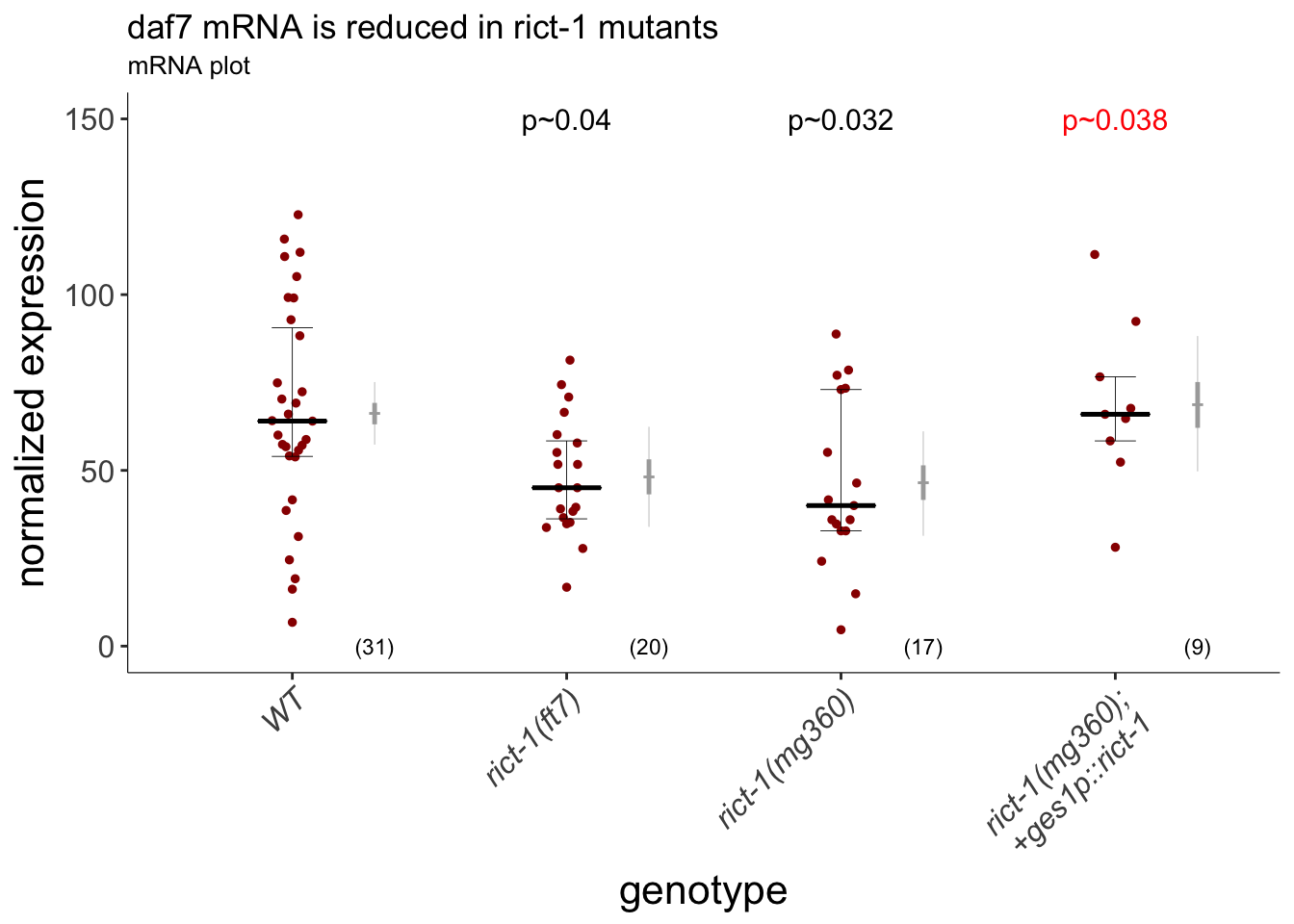
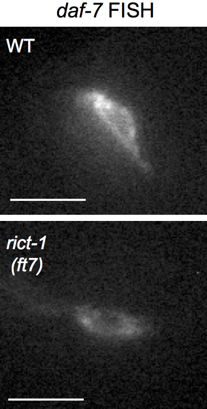
Figure 2B daf-7 mRNA is reduced in rict-1 mutants. Intestinal expression of rict-1 using the intestinal ges-1 promoter rescues daf-7 expression. Quantification of daf-7 mRNA levels in ASI assessed via fluorescent in situ hybridization. Expression was normalized by subtracting mean background pixel values for each image. Each dot is the fluorescence intensity in a single ASI neuron; numbers in parentheses below indicate the number of neurons examined in 3 independent pooled experiments. Horizontal thick bar indicates median. Error bars are quartiles. Light gray thin and thick vertical bars at right indicate Bayesian 95% and 75% credible intervals, respectively. P-values of differences relative to wild-type and rict-1(mg360) animals are indicated in black and red, respectively. For rict-1(mg360) and rict-1(ft7), p~0.04 and p~0.032 compared to N2, respectively. For ges-1 rescue, p~0.038 compared to rict-1(ft7). n=2 independent experiments, pooled data. 2 outlier data points were removed in total. P-values of differences in means relative to wild-type and corresponding mutant animals are indicated in black and red, respectively.
library(sjPlot)
sjt.lm(lm.1, depvar.labels = "mean mRNA levels (AU)", show.se = TRUE, show.fstat = TRUE)
|
|
|
mean mRNA levels (AU)
|
|
|
|
B
|
CI
|
std. Error
|
p
|
|
(Intercept)
|
|
66.41
|
57.31 – 75.51
|
4.57
|
<.001
|
|
genotype
|
|
ft7
|
|
-18.33
|
-32.87 – -3.80
|
7.29
|
.014
|
|
mg360
|
|
-19.95
|
-35.24 – -4.65
|
7.67
|
.011
|
|
mg360resc
|
|
2.22
|
-16.97 – 21.41
|
9.63
|
.819
|
|
Observations
|
|
77
|
|
R2 / adj. R2
|
|
.136 / .100
|
|
F-statistics
|
|
3.826*
|
knitr::kable(contrasts, caption="Pairwise comparisons from ANOVA (Dunnett)")
Pairwise comparisons from ANOVA (Dunnett)
| ft7 - N2 |
-18.334597 |
7.293687 |
73 |
-2.5137625 |
0.0400051 |
p~0.04 |
| mg360 - N2 |
-19.946391 |
7.674908 |
73 |
-2.5989094 |
0.0321795 |
p~0.032 |
| mg360resc - N2 |
2.216681 |
9.629102 |
73 |
0.2302064 |
0.9930260 |
p~1 |
knitr::kable(mixed[,c(6,1:5)], caption = "Bayesian credible intervals")
Bayesian credible intervals
| N2 |
66.21063 |
57.33521 |
75.12330 |
63.10270 |
69.20060 |
| ft7 |
48.13964 |
33.93267 |
62.40929 |
43.18285 |
53.14452 |
| mg360 |
46.48935 |
31.39981 |
61.11334 |
41.59141 |
51.43346 |
| mg360resc |
68.68817 |
49.71407 |
88.23230 |
62.10228 |
75.13613 |
2C
#days = as.factor(8:10) # days containing N2 and ft7 27º data
dates = c("12_1_16",  "12_20_17", "12_21_17", "12_6_16",  "9_21_16" )
strains = c("N2", "ft7", "ft7exifb2", "ft7exgpa4")
foods = "OP50"
d28<-read.csv('extdata/2C_Daf28GFP_rescue.csv') %>%
separate(ID, c("ID.A", "ID.B"), sep = ":", extra = "drop") %>%
  subset(mean!=4095 & food == foods & temp == "27" & genotype %in% strains & pheromone == 0) %>%
  mutate(genotype = factor(genotype, levels = strains),
         genoID = interaction(date,genotype, ID.A)
         )

df <- d28 %>% group_by(neuron,date,genotype,genoID) %>%
  summarise(cell.norm = mean(mean, na.rm = TRUE)) %>%
  data.frame() %>%
  mutate(group.id = interaction(genotype, neuron),
         dataset = case_when(
           date %in% c("12_1_16","12_6_16","9_21_16") ~ "3C_3D",
           date %in% c("12_20_17", "12_21_17") ~ "_new"
         )) # take mean of each worm
day.means <- df %>%
  filter(genotype == "ft7") %>%
  group_by(date,neuron) %>%
  summarise(mean_ft7 = mean(cell.norm)) %>% data.frame()

#normalize to mean rict-1 mutant ASJ value per day
df %<>% mutate(cell.norm =
                 case_when(
                   neuron == "ASI" ~ case_when(
                     date == dates[1] ~ (cell.norm * day.means[2,3]) / day.means[2,3],
                     date == dates[2] ~ (cell.norm * day.means[2,3]) / day.means[4,3],
                     date == dates[3] ~ (cell.norm * day.means[2,3]) / day.means[6,3],
                     date == dates[4] ~ (cell.norm * day.means[2,3]) / day.means[8,3],
                     date == dates[5] ~ (cell.norm * day.means[2,3]) / day.means[10,3]
                   ),
                   neuron == "ASJ" ~ case_when(
                     date == dates[1] ~ cell.norm,
                     date == dates[2] ~ (cell.norm * day.means[2,3]) / day.means[4,3],
                     date == dates[3] ~ (cell.norm * day.means[2,3]) / day.means[6,3],
                     date == dates[4] ~ (cell.norm * day.means[2,3]) / day.means[8,3],
                     date == dates[5] ~ (cell.norm * day.means[2,3]) / day.means[10,3]
                   )
                 )
)


#fit simple linmod to est outliers:
log.tran<-lsmeans::make.tran(type="genlog", param = c(0,10)) #make log10 transformation
lm1 <- with(log.tran, lm(linkfun(cell.norm) ~ neuron * genotype, data = df))
df %<>% flag_outliers(lin.mod=lm1, threshold = 4, df = ., noplot=TRUE)

# linear MM
lm <- with(log.tran, lm(linkfun(cell.norm) ~ neuron * genotype, data = df[df$outlier.status==FALSE,]))
stanlmer <- with(log.tran, stan_lmer(linkfun(cell.norm) ~ 1 + group.id + (1|date) + (1:group.id:date), data = df[df$outlier.status==FALSE,]))


contrasts<-summary(lsmeans::lsmeans(lm, pairwise ~ genotype | neuron)$contrasts) %>% dauergut::prange()
mixed <- stanlmer %>% getStan_CIs(type = "log", group = "neuron", base = 10, compare_gt = TRUE) %>%
  mutate(x.pos = rep(c(1.3,2.3,3.3,4.3),2))
plot.contrasts<-c("",contrasts$prange[1:3],
                  "",contrasts$prange[7:9])
plot.contrasts.2<-c("","",contrasts$prange[4:5],
                    "","",contrasts$prange[10:11])

labels <- c("WT",
            "rict-1(ft7)",
            "rict-1(ft7); +ifb2p::rict-1",
            "rict-1(ft7); +gpa4p::rict-1") %>% stringr::str_wrap(width = 10)
#plot
p <- df %>%
  ggplot(aes(x=genotype, y = cell.norm)) +
  geom_quasirandom(aes(y=cell.norm, pch = dataset),cex=1,colour = "#339900",
                           width = 0.075,size=0.3,
                           method = 'smiley') +
  theme_my +
  guides(pch=FALSE) +
  list(dauergut::add.median(width = 0.25), dauergut::add.quartiles()) +
  labs(title = "daf-28 is also reduced in rict-1 mutants",
           y = "mean GFP intensity", x="genotype") +
  stat_summary(aes(x=genotype, group = genotype, y = 3000), geom="text", fun.data=box_annot,
                    label=plot.contrasts, size = 4) +
  stat_summary(aes(x=genotype, group = genotype, y = 2800), geom="text", fun.data=box_annot,
                    label=plot.contrasts.2, size = 4, colour = "red") +
  geom_errorbar(data=mixed, aes(x=x.pos,y=mean, ymin=lower.CL, ymax=upper.CL),
                     width=0,colour ="grey", lwd=0.15) +
  geom_errorbar(data=mixed, aes(x=x.pos,y=mean, ymin = lower.25, ymax = upper.75),
                     width=0,colour = "darkgrey", lwd = 0.15+0.7) +
  stat_summary(aes(x=as.numeric(as.factor(genotype)) + 0.3,y=0,group = genotype),
                    fun.data = fun_length, geom = "text",size = 4) +
  facet_grid(.~neuron) +
  scale_x_discrete(labels = labels) +
  theme(strip.background = element_blank(),
        strip.text = element_text(size = 16,face="bold"),
        axis.text.y = element_text(size=12),
        axis.text.x = element_text(size = 12, face = "italic"),
        axis.title = element_text(size=16),
        panel.spacing.x=unit(2,"lines"))

#image of daf-28 GFP
img.path <- file.path(pathname,"figures","2D_daf-28GFP.png")
include_graphics(img.path)
p
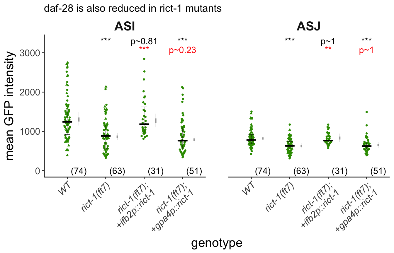
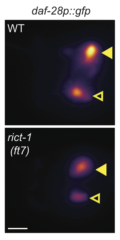
Figure 2C (Left) Representative images of daf-28p::gfp expression in one of the bilateral and ASI and ASJ neurons in animals of the indicated genotypes. Yellow filled and open arrowheads indicate ASI and ASJ soma, respectively. Anterior is at left. Scale bar: 5 μm. (Right) Quantification of daf-28p::gfp expression in ASI and ASJ. Each dot is the mean fluorescence intensity in a single animal (2 neurons per animal); numbers in parentheses below indicate the number of animals examined in 3 independent experiments. Horizontal thick bar indicates median. Error bars are quartiles. Light gray thin and thick vertical bars at right indicate Bayesian 95% and 75% credible intervals, respectively. ** and *** - different from wild-type at P<0.01 and P<0.001, respectively; (ANOVA with Tukey-type multivariate-t post-hoc adjustment).
library(sjPlot)
sjt.lm(lm, depvar.labels = "log(mean GFP intensity) (AU)", show.se = TRUE, show.fstat = TRUE)
|
|
|
log(mean GFP intensity) (AU)
|
|
|
|
B
|
CI
|
std. Error
|
p
|
|
(Intercept)
|
|
3.11
|
3.08 – 3.14
|
0.02
|
<.001
|
|
neuronASJ
|
|
-0.21
|
-0.25 – -0.16
|
0.02
|
<.001
|
|
genotype
|
|
genotypeft7
|
|
-0.18
|
-0.23 – -0.13
|
0.02
|
<.001
|
|
genotypeft7exifb2
|
|
-0.03
|
-0.09 – 0.03
|
0.03
|
.370
|
|
genotypeft7exgpa4
|
|
-0.23
|
-0.28 – -0.18
|
0.03
|
<.001
|
|
neuronASJ:genotypeft7
|
|
0.07
|
0.00 – 0.14
|
0.03
|
.035
|
|
neuronASJ:genotypeft7exifb2
|
|
0.02
|
-0.06 – 0.10
|
0.04
|
.628
|
|
neuronASJ:genotypeft7exgpa4
|
|
0.12
|
0.05 – 0.19
|
0.04
|
<.001
|
|
Observations
|
|
417
|
|
R2 / adj. R2
|
|
.414 / .404
|
|
F-statistics
|
|
41.338***
|
knitr::kable(mixed[,c(6,1:5)], caption = "Bayesian credible intervals")
Bayesian credible intervals
| N2 |
1301.3384 |
1148.9742 |
1489.3897 |
1250.0170 |
1352.2357 |
| ft7 |
862.4539 |
772.5949 |
958.8130 |
831.5989 |
894.1867 |
| ft7exifb2 |
1266.9316 |
1101.7595 |
1451.5025 |
1208.5608 |
1328.6941 |
| ft7exgpa4 |
787.6103 |
697.6164 |
889.1113 |
756.4258 |
820.4525 |
| N2 |
817.6985 |
741.5358 |
903.8321 |
790.1152 |
845.6063 |
| ft7 |
631.5011 |
567.3274 |
702.9728 |
608.7091 |
654.9188 |
| ft7exifb2 |
827.4752 |
725.4745 |
943.1699 |
791.3480 |
866.3178 |
| ft7exgpa4 |
648.9093 |
576.9041 |
728.6359 |
624.7360 |
674.9000 |
knitr::kable(contrasts, caption = "pairwise comparisons (Tukey)")
pairwise comparisons (Tukey)
| N2 - ft7 |
ASI |
0.1812272 |
0.0240311 |
409 |
7.5413602 |
0.0000000 |
*** |
| N2 - ft7exifb2 |
ASI |
0.0266916 |
0.0297459 |
409 |
0.8973202 |
0.8062379 |
p~0.81 |
| N2 - ft7exgpa4 |
ASI |
0.2331576 |
0.0260984 |
409 |
8.9337827 |
0.0000000 |
*** |
| ft7 - ft7exifb2 |
ASI |
-0.1545355 |
0.0307235 |
409 |
-5.0298767 |
0.0000044 |
*** |
| ft7 - ft7exgpa4 |
ASI |
0.0519304 |
0.0272074 |
409 |
1.9086898 |
0.2259441 |
p~0.23 |
| ft7exifb2 - ft7exgpa4 |
ASI |
0.2064660 |
0.0323662 |
409 |
6.3790679 |
0.0000000 |
*** |
| N2 - ft7 |
ASJ |
0.1108181 |
0.0230904 |
409 |
4.7993066 |
0.0000133 |
*** |
| N2 - ft7exifb2 |
ASJ |
0.0066176 |
0.0288175 |
409 |
0.2296397 |
0.9957282 |
p~1 |
| N2 - ft7exgpa4 |
ASJ |
0.1115180 |
0.0246586 |
409 |
4.5224807 |
0.0000473 |
*** |
| ft7 - ft7exifb2 |
ASJ |
-0.1042005 |
0.0295509 |
409 |
-3.5261338 |
0.0026362 |
** |
| ft7 - ft7exgpa4 |
ASJ |
0.0006998 |
0.0255119 |
409 |
0.0274322 |
0.9999926 |
p~1 |
| ft7exifb2 - ft7exgpa4 |
ASJ |
0.1049004 |
0.0307918 |
409 |
3.4067640 |
0.0040134 |
** |
2D
strains<-c("N2", "rict-1(mg360)", "rict-1(ft7)")
#dates<-c("12_5_14", "12_19_14", "1_19_15","3_22_14", "2_25_14", "4_11_14")
dates<-c("12_5_14", "12_19_14","3_22_14", "2_25_14", "4_11_14")
foods <- c("OP50", "HB101")
rict1.food<-read.csv(file.path(pathname, "extdata", "1B_2D_rict-1_TORC2.csv"), header=TRUE) %>% format_dauer(p.dauer = "exclude") %>%
  dplyr::filter(day %in% dates) %>% mutate(logit.p = car::logit(pct, adjust=0.01),
                                           plate.ID = interaction(food, plateID))

# rict1.food %>% ggplot(aes(x=food, y=pct)) + geom_boxplot() + stat_summary(aes(y=pct, group=day, colour = day), fun.y = mean, geom = "line") + facet_grid(.~genotype)

#lm
lm.add <- lm(pct ~ genotype + food, data = rict1.food)
lm.int <- update(lm.add,.~. + genotype*food)
#stan
rict.food.groups <- rict1.food %>% mutate(group.id = interaction(genotype, food))
stan.glmm <- run_dauer_stan(df = rict.food.groups, type="dauer-grouped", group = "food", intercept = FALSE)
contrasts<-dauergut::dunnett_contrasts(lm.int, ref.index = 1, factor = "genotype", interaction = "food")
mixed<-dauergut::getStan_CIs(stan.glmm, type="dauer", group = "food", intercept = FALSE)

plot.contrasts <- c("",contrasts$interaction$prange[1], "", contrasts$interaction$prange[2], "", contrasts$interaction$prange[3])
plot.contrasts.interaction <- summary(lm.int)$coefficients[,4][5:6] %>% data.frame() %>% mutate(p.value = c(.[[1]],.[[2]]), genotype = strains[2:3]) %>% dauergut::prange()

index<-rep(seq_len(length(strains)), each = 2)

plot.contrasts.H0 <- data.frame(cbind(food = foods, genotype = strains[index])) %>%
  mutate(prange = plot.contrasts)

(p<-ggplot(rict1.food, aes(x=food)) +
  stat_summary(aes(y=pct, group=day), colour = "black", fun.y = mean, geom = "line", alpha = 0.2, linetype = 2) +
  add.median.dauer() +
  add.Bayes.CI() +
  geom_dotplot(aes(y=pct, colour = food, fill=food),binwidth=.015, binaxis="y", position="dodge", stackdir="center", size =.3) +
    #geom_point(aes(y=pct,colour = food), size = 0.7, alpha = 0.75) +
  labs(title = "rict-1 mutants are deficient in food suppression",
           y = "proportion dauer",
           x = "food") +
  facet_grid(.~genotype, switch="both") +
  scale_colour_manual(values = c("black", "#FF9933")) +
    scale_fill_manual(values = c("black", "#FF9933")) +
      scale_y_continuous(breaks=c(0,0.25,0.5,0.75, 1.0)) +
      scale_x_discrete(labels=function(x) sub(" ","\n",x,fixed=TRUE)) +
  geom_text(data = plot.contrasts.H0, aes(x=2, label = prange, y = 1.075, group = NULL), size = 4) +
    stat_summary(aes(x=as.numeric(as.factor(food)) + 0.3, y=-0.05),
                   fun.data = fun_length, geom = "text", size = 3) +
  theme_classic() +
    theme(strip.text.x = element_text(size = 12, face="italic"),
      axis.text.x = element_blank(),
          axis.text.y = element_text(size = 12),
          axis.line = element_line(size=0.2),
          axis.title = element_text(size=16)))
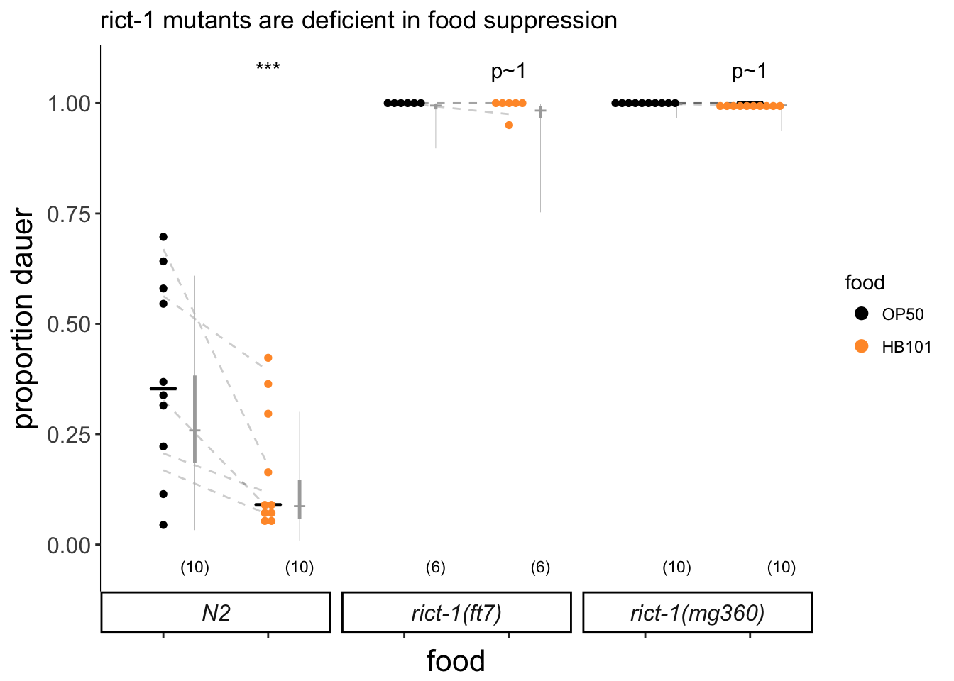
Figure 2D
rict-1 mutants are deficient in food suppression of dauer formation. Dauers formed by wild-type and rict-1 mutants on OP50 or HB101 at 27°C. Each black dot indicates the average number of dauers formed in a single assay. Horizontal black bar indicates median. Light gray thin and thick vertical bars at right indicate Bayesian 95% and 75% credible intervals, respectively. Numbers in parentheses below indicate the number of independent experiments with at least 19 animals scored in each. Dashed lines indicate mean change in dauer formation per experimental day. P-values are with respect to growth on OP50; *** - different from growth on OP50 at P<0.001 [two-factor ANOVA with F(5.21) with 2 Df, P=0.0092 for genotype*food interaction, Tukey-type multivariate-t post-hoc adjustment].
library(sjPlot)
sjt.lm(lm.int, depvar.labels = "proportion of dauers", show.fstat = TRUE)
|
|
|
proportion of dauers
|
|
|
|
B
|
CI
|
p
|
|
(Intercept)
|
|
0.39
|
0.31 – 0.46
|
<.001
|
|
genotype
|
|
genotyperict-1(mg360)
|
|
0.61
|
0.51 – 0.72
|
<.001
|
|
genotyperict-1(ft7)
|
|
0.61
|
0.49 – 0.73
|
<.001
|
|
foodHB101
|
|
-0.22
|
-0.32 – -0.11
|
<.001
|
|
genotyperict-1(mg360):foodHB101
|
|
0.22
|
0.07 – 0.37
|
.005
|
|
genotyperict-1(ft7):foodHB101
|
|
0.21
|
0.04 – 0.38
|
.017
|
|
Observations
|
|
52
|
|
R2 / adj. R2
|
|
.913 / .904
|
|
F-statistics
|
|
97.027***
|
knitr::kable(contrasts[1], caption = "pairwise comparisons by genotype (ANOVA)")
pairwise comparisons by genotype (ANOVA)
| rict-1(mg360) - N2 |
0.7222366 |
0.0369869 |
46 |
19.52681 |
0 |
*** |
| rict-1(ft7) - N2 |
0.7187193 |
0.0427088 |
46 |
16.82836 |
0 |
*** |
|
knitr::kable(contrasts[2], caption = "pairwise comparisons by food (ANOVA)")
pairwise comparisons by food (ANOVA)
| OP50 - HB101 |
N2 |
0.2190433 |
0.0523074 |
46 |
4.1876156 |
0.0003762 |
*** |
| OP50 - HB101 |
rict-1(mg360) |
0.0012987 |
0.0523074 |
46 |
0.0248282 |
0.9999921 |
p~1 |
| OP50 - HB101 |
rict-1(ft7) |
0.0083333 |
0.0675286 |
46 |
0.1234045 |
0.9990374 |
p~1 |
|
S1A
include_graphics(file.path(pathname, "figures","S1A_daf7FISH.png"))
S1B
strains<-c("N2","mg360")
conc.adjust <-15
dates<-c("8_10_16")
d7GFP<-read.csv(file.path(pathname,"extdata","2A_3A_daf7GFP.csv")) %>% filter(mean!=4095 & genotype %in% strains & date %in% dates & temp == "25" & food == "OP50") %>% mutate(genotype = factor(genotype, levels=strains), ID = as.character(ID)) %>%
  separate(ID, c("ID.A", "ID.B"), sep = ":", extra = "drop") %>%
  mutate(genoID = paste(date, genotype, ID.A, sep = ":"), cell.norm = mean, adj.pheromone = pheromone + conc.adjust,
         inv.pher = 1/adj.pheromone) #genoID is animal, 2 cells per animal measured.

df <- d7GFP %>% group_by(date, genotype, genoID, adj.pheromone) %>% summarise(cell.norm = mean(cell.norm))

log.tran<-lsmeans::make.tran(type="genlog", param = c(0,10))

#convert to proportion:
lm <- lm(cell.norm ~ genotype + adj.pheromone,  data = df)
lm1<- lm(cell.norm ~ genotype + poly(adj.pheromone,2),  data = df)
lm2 <- lm(cell.norm ~ genotype * poly(adj.pheromone, 2), data = df)

# stanlmer <- with(log.tran, rstanarm::stan_lmer(linkfun(cell.norm) ~ genotype + (1|date) + (1:genotype:date),
#                                                data = df,
#                                                chains = 3,
#                                                cores =4,
#                                                seed = 2000,
#                                                iter=6000,
#                                                control = list(adapt_delta=0.99)))


newdata = data.frame(genotype = rep(strains, each = 241), adj.pheromone = rep(seq(10,2410, by = 10),2),genoID = rep(0, 482))

### for non-interaction ###
#glm.simple <- glm(data = rictC3, cbind(dauer, non) ~ concentration.uM. + genotype, family = binomial)
predictions <- predict(lm, newdata = newdata, type = "response", se.fit = TRUE)
predictions.2 <- predict(lm2, newdata = newdata, type = "response", se.fit = TRUE)
newdata1 <- cbind(newdata, predictions.2)
newdata1 %<>% mutate(lower = (fit - se.fit), upper = (fit + se.fit), AU = fit, genotype = factor(genotype, levels = strains))


(p<-df %>% ungroup %>% ggplot(aes(x= adj.pheromone)) +
    geom_ribbon(data = newdata1,aes(ymin=lower, ymax=upper, fill=genotype), alpha=0.3) +
    geom_line(data = newdata1,aes(x =  adj.pheromone, y = AU, colour = genotype)) +
    add.median(width = 150) +
    add.quartiles(width = 60) +
    geom_quasirandom(aes(y=cell.norm),colour = "#339900", cex=1,
                           width = 40,size=0.3,
                           method = 'smiley') +
    labs(y = "GFP intensity (AU)",
         x = "ascr#5 concentration (nM)") +
    facet_grid(.~genotype) +
    scale_fill_manual(values = c("grey", "lightblue")) +
    scale_colour_manual(values = c("grey", "lightblue")) +
  geom_text(aes(y = 1.075, x= adj.pheromone), label = "") +
  theme_classic() +
  theme(
        axis.text.x=element_text(angle=45, hjust=1, size=12),
        axis.text.y = element_text(size=16),
        axis.title.y = element_text(size =20),
        axis.title.x = element_text(size=16),
        strip.text.x = element_blank(),
        panel.spacing = unit(2,"lines")) +
    stat_summary(aes(x= adj.pheromone + 0.3, y=-.025),
                      fun.data = fun_length, geom = "text", size = 4))
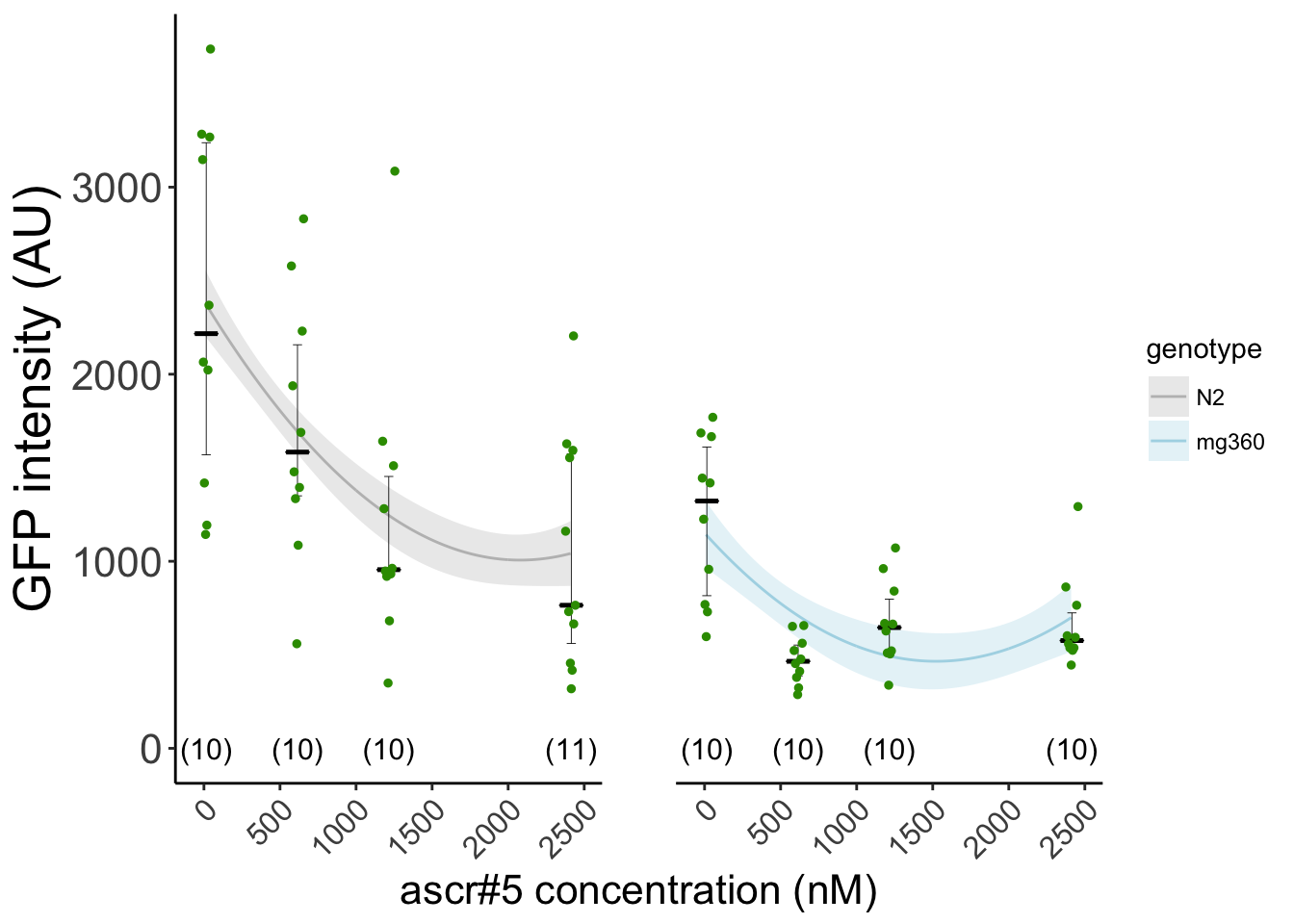
Figure S1B rict-1 mutants show enhanced response to pheromone ascr#5. daf-7::GFP expression in wild-type (black) and rict-1(mg360) (blue) animals at 25°C in the presence of the indicated concentrations of ascr#5 and live OP50. Each dot indicates the average ASI GFP intensity in each each animal (2 neurons per animal). Horizontal bar indicates median, error bars indicate quartiles. The number of animals are indicated in parentheses. Lines indicate predictions from quadratic fit.
library(sjPlot)
sjt.lm(lm2, depvar.labels = "proportion of dauers", show.se = TRUE, show.fstat = TRUE)
|
|
|
proportion of dauers
|
|
|
|
B
|
CI
|
std. Error
|
p
|
|
(Intercept)
|
|
1581.53
|
1400.91 – 1762.16
|
90.67
|
<.001
|
|
genotypemg360
|
|
-821.95
|
-1078.99 – -564.91
|
129.03
|
<.001
|
|
poly(adj.pheromone, 2)1
|
|
-4209.77
|
-5823.52 – -2596.03
|
810.07
|
<.001
|
|
poly(adj.pheromone, 2)2
|
|
1838.23
|
208.73 – 3467.72
|
817.98
|
.028
|
|
genotypemg360:poly(adj.pheromone, 2)1
|
|
2975.46
|
661.29 – 5289.64
|
1161.67
|
.012
|
|
genotypemg360:poly(adj.pheromone, 2)2
|
|
-141.83
|
-2454.91 – 2171.25
|
1161.12
|
.903
|
|
Observations
|
|
81
|
|
R2 / adj. R2
|
|
.510 / .478
|
|
F-statistics
|
|
15.629***
|
S1C
strains <- c("N2", "rict-1(ft7)")
foods <- "OP50"
rictC3 <- read.csv(file.path(pathname, 'extdata','S1C_rict1Pheromone.csv')) %>% format_dauer(p.dauer = "exclude") %>% mutate(plateID = interaction(plateID,concentration.uM.))

# for glm fit
glm <- glm(data = rictC3, cbind(dauer, non) ~ concentration.uM. + genotype + concentration.uM. * genotype, family = binomial)

newdata = data.frame(genotype = rep(strains, each = 241), concentration.uM. = rep(seq(0,2.4, by = 0.01),2),plateID = rep(0, 482), n = rep(60, 482))

### for non-interaction ###
glm.simple <- glm(data = rictC3, cbind(dauer, non) ~ concentration.uM. + genotype, family = binomial)
predictions <- predict(glm, newdata = newdata, type = "response", se.fit = TRUE)
newdata1 <- cbind(newdata, predictions)
newdata1 %<>% mutate(lower = (fit - se.fit), upper = (fit + se.fit), pct = fit)


(p<-rictC3 %>% ggplot(aes(x=concentration.uM.,y = pct)) +
  geom_ribbon(data = newdata1,aes(ymin=lower, ymax=upper,fill=genotype), alpha=0.3) +
  geom_line(data = newdata1,aes(x = concentration.uM., y = pct, colour = genotype)) +
  geom_point(aes(y=pct), size = 0.6, alpha = 0.75) +
  add.median.dauer() +
  labs(y = "proportion dauer",
       x = "ascr#5 concentration (uM)") +
  facet_grid(.~genotype) +
  scale_fill_manual(values = c("grey", "lightblue")) +
  scale_colour_manual(values = c("grey", "lightblue")) +
  geom_text(aes(y = 1.075, x=concentration.uM.), label = "") +
    coord_cartesian(ylim = c(-.005,1.075)) +
      scale_y_continuous(breaks=c(0,0.25,0.5,0.75,1)) +
  theme_classic() +
  theme(
        axis.text.x = element_text(size=16),
        axis.text.y = element_text(size=16),
        axis.title.y = element_text(size =20),
        axis.title.x = element_text(size=16),
        strip.text.x = element_blank(),
        panel.spacing = unit(2,"lines")) +
    stat_summary(aes(x=concentration.uM. + 0.3, y=-.025),
                      fun.data = fun_length, geom = "text", size = 4)
)
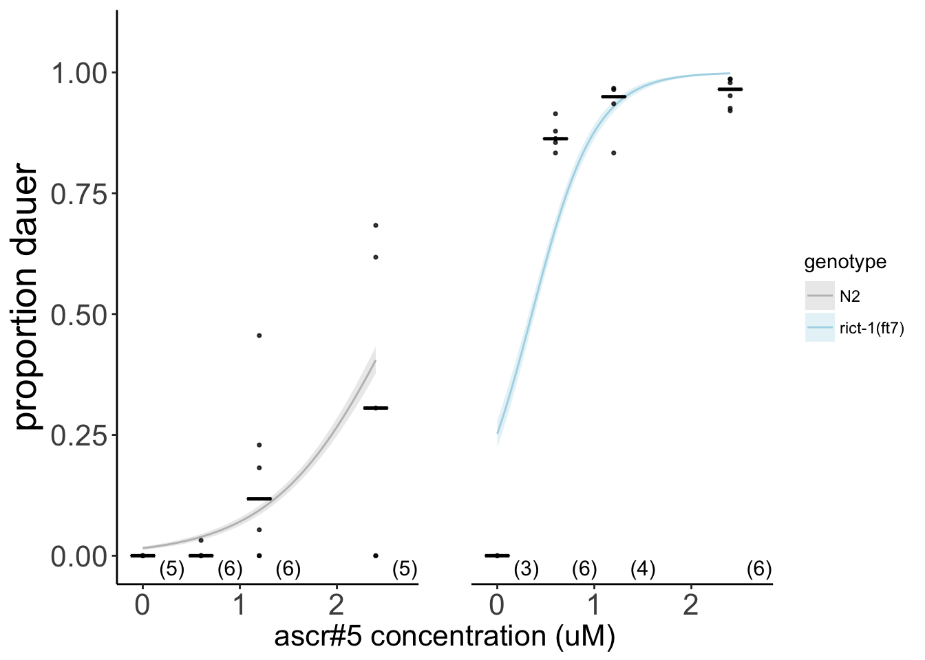
Figure S1C rict-1 mutants show enhanced response to pheromone ascr#5. Dauers formed by wild-type (black) and rict-1(ft7) (blue) animals at 25°C in the presence of the indicated concentrations of ascr#5. Each dot indicates the proportion of dauers formed in a single assay. Horizontal bar indicates median. Numbers in parentheses below indicate the number of independent experiments with at least 27 animals each. Lines indicate predictions from GLM fit, corresponding to an odds ratio of as.numeric(round(exp(coef(glm))[3],1)) for rict-1 across this range of ascr#5 concentrations.
library(sjPlot)
sjt.glm(glm, depvar.labels = "proportion of dauers", show.se = TRUE, show.chi2 = TRUE)
|
|
|
proportion of dauers
|
|
|
|
Odds Ratio
|
CI
|
std. Error
|
p
|
|
(Intercept)
|
|
0.02
|
0.01 – 0.02
|
0.00
|
<.001
|
|
concentration.uM.
|
|
4.79
|
3.83 – 6.05
|
0.56
|
<.001
|
|
genotyperict-1(ft7)
|
|
21.28
|
12.69 – 36.47
|
5.72
|
<.001
|
|
concentration.uM.:genotyperict-1(ft7)
|
|
4.41
|
2.73 – 7.35
|
1.11
|
<.001
|
|
Observations
|
|
41
|
|
Χ2deviance
|
|
p=.000
|
S1D
foods <- "OP50"
strains<-c("N2","rict-1(ft7)","rict-1(ft7); ex[ASI::daf7]","rict-1(ft7); ex[ASI::daf28]","rict-1(ft7); ex[ASJ::daf28]")
daf7supp<-read.csv(file.path(pathname, "extdata","S1D_daf7_daf28_suppression.csv")) %>% format_dauer(p.dauer = "non")

# daf7supp$genotype<- factor(daf7supp$genotype, levels = strains)
# daf7supp$pct<-as.numeric(paste(daf7supp$dauer/(daf7supp$dauer+daf7supp$pd + daf7supp$non))) #omitted arrest
# daf7supp$non.dauer<-as.numeric(paste(daf7supp$pd+daf7supp$non))

lm <- daf7supp %>% dauer_ANOVA()
#stan
stan.glmm <- daf7supp %>% dauergut::run_dauer_stan()
foods <- "OP50"
contrasts<-dauergut::tukey_contrasts(lm, "genotype")
mixed<-stan.glmm %>% dauergut::getStan_CIs(type = "dauer")
plot.contrasts<-c("",contrasts$prange[1],"","","")
plot.contrasts.2<-c("", "", contrasts$prange[5:7]) #for rescue vs rict-1

labels <- c("WT","rict-1(ft7)","rict-1(ft7); +ASIp::daf-7","rict-1(ft7); +ASIp::daf-28","rict-1(ft7); +ASJp::daf-28") %>% stringr::str_wrap(width = 10)


p<-dauergut::plot_CIs(daf7supp, title='daf-7 expression in ASI suppresses rict-1 dauer phenotype', plot.contrasts, plot.contrasts.2, ypos = 1.075, offset = 0, type = "dauer", labels = labels)
p
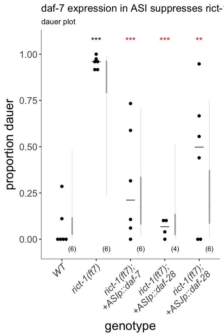
Figure 2C Expression of daf-7 in ASI or daf-28 in ASI or ASJ suppressed aberrent dauer formation in rict-1 mutants. Dauers formed by animals of the indicated genotypes at 27°C. Each black dot indicates the average number of dauers formed in a single assay. Horizontal black bar indicates median. Light gray thin and thick vertical bars at right indicate Bayesian 95% and 75% credible intervals, respectively. Numbers in parentheses below indicate the number of independent experiments with at least 36 and 9 animals each scored for non-transgenic and transgenic animals, respectively. Promoters driving expression in ASI and ASJ were srg-47p and trx-1p, respectively. One transgenic line was tested for each condition. *** - different from wild-type at P<0.001; ** and *** - different from rict-1(ft7) at P<0.01 and P<0.001, respectively (ANOVA with Tukey-type multivariate-t post-hoc adjustment). P-values of differences in means relative to wild-type and corresponding mutant animals are indicated in black and red, respectively.
library(sjPlot)
sjt.lm(lm, depvar.labels = "proportion of dauers", show.se = TRUE, show.fstat = TRUE)
|
|
|
proportion of dauers
|
|
|
|
B
|
CI
|
std. Error
|
p
|
|
(Intercept)
|
|
0.07
|
-0.13 – 0.26
|
0.09
|
.493
|
|
genotype
|
|
rict-1(ft7)
|
|
0.89
|
0.61 – 1.17
|
0.13
|
<.001
|
|
rict-1(ft7); ex[ASI::daf7]
|
|
0.23
|
-0.04 – 0.51
|
0.13
|
.094
|
|
rict-1(ft7); ex[ASI::daf28]
|
|
-0.01
|
-0.32 – 0.31
|
0.15
|
.971
|
|
rict-1(ft7); ex[ASJ::daf28]
|
|
0.37
|
0.09 – 0.65
|
0.13
|
.012
|
|
Observations
|
|
28
|
|
R2 / adj. R2
|
|
.709 / .658
|
|
F-statistics
|
|
14.007***
|
knitr::kable(contrasts, caption="Pairwise comparisons from ANOVA (Tukey)")
Pairwise comparisons from ANOVA (Tukey)
| N2 - rict-1(ft7) |
-0.8882755 |
0.1343472 |
23 |
-6.6117898 |
0.0000052 |
*** |
| N2 - rict-1(ft7); ex[ASI::daf7] |
-0.2347136 |
0.1343472 |
23 |
-1.7470673 |
0.4258378 |
p~0.43 |
| N2 - rict-1(ft7); ex[ASI::daf28] |
0.0055423 |
0.1502047 |
23 |
0.0368985 |
0.9999995 |
p~1 |
| N2 - rict-1(ft7); ex[ASJ::daf28] |
-0.3687942 |
0.1343472 |
23 |
-2.7450829 |
0.0771804 |
p~0.077 |
| rict-1(ft7) - rict-1(ft7); ex[ASI::daf7] |
0.6535619 |
0.1343472 |
23 |
4.8647225 |
0.0005637 |
*** |
| rict-1(ft7) - rict-1(ft7); ex[ASI::daf28] |
0.8938178 |
0.1502047 |
23 |
5.9506630 |
0.0000476 |
*** |
| rict-1(ft7) - rict-1(ft7); ex[ASJ::daf28] |
0.5194813 |
0.1343472 |
23 |
3.8667069 |
0.0062462 |
** |
| rict-1(ft7); ex[ASI::daf7] - rict-1(ft7); ex[ASI::daf28] |
0.2402559 |
0.1502047 |
23 |
1.5995230 |
0.5114687 |
p~0.51 |
| rict-1(ft7); ex[ASI::daf7] - rict-1(ft7); ex[ASJ::daf28] |
-0.1340806 |
0.1343472 |
23 |
-0.9980156 |
0.8530372 |
p~0.85 |
| rict-1(ft7); ex[ASI::daf28] - rict-1(ft7); ex[ASJ::daf28] |
-0.3743365 |
0.1502047 |
23 |
-2.4921752 |
0.1268946 |
p~0.127 |
knitr::kable(mixed[,c(6,1:5)], caption = "Bayesian credible intervals")
Bayesian credible intervals
| N2 |
0.0555770 |
0.0033152 |
0.4805341 |
0.0243011 |
0.1180252 |
| rict-1(ft7) |
0.9039164 |
0.2329556 |
0.9928633 |
0.7897794 |
0.9654116 |
| rict-1(ft7); ex[ASI::daf7] |
0.1713925 |
0.0118883 |
0.7096820 |
0.0797292 |
0.3378971 |
| rict-1(ft7); ex[ASI::daf28] |
0.0551065 |
0.0027477 |
0.5148130 |
0.0218284 |
0.1371370 |
| rict-1(ft7); ex[ASJ::daf28] |
0.1811430 |
0.0092616 |
0.7501988 |
0.0838653 |
0.3739147 |
S1E
strains<-c("N2","rict-1(mg360)","rict-1;daf-16")
foods <- "OP50"
daf16supp<-read.csv(file.path(pathname, "extdata","S1E_daf16_suppression.csv")) %>% format_dauer(.,p.dauer = "dauer")

# daf28supp$genotype<- factor(daf28supp$genotype, levels = strains)
# daf28supp$pct<-as.numeric(paste(daf28supp$dauer/(daf28supp$dauer+daf28supp$pd + daf28supp$non))) #omitted arrest
# daf28supp$non.dauer<-as.numeric(paste(daf28supp$pd+daf28supp$non))
lm <- daf16supp %>% dauer_ANOVA()
#stan
stan.glmm <- daf16supp %>% stan_glmer(formula = cbind((dauer+pd), (n-(dauer+pd))) ~ genotype + (1|day) + (1|strainDate) + (1|plateID),
                       data=.,
                       family = binomial(link="logit"),
                       chains = 3, cores =4, seed = 2000,iter=6000,
                       control = list(adapt_delta=0.99))
contrasts<-dauergut::tukey_contrasts(lm, "genotype")
mixed<-stan.glmm %>% getStan_CIs(type="dauer")
plot.contrasts<-c("",contrasts$prange[1],"")
plot.contrasts.2<-c("", "", contrasts$prange[3]) #for rescue vs rict-1

labels <- c("WT","rict-1(mg360)","daf-16(mu86; rict-1(mg360)") %>% stringr::str_wrap(width = 10)

p<-dauergut::plot_CIs(daf16supp, title='rict-1 acts in the insulin pathway to inhibit dauer formation', plot.contrasts, plot.contrasts.2, ypos = 1.075, offset = 0, type = "dauer", labels = labels)
p
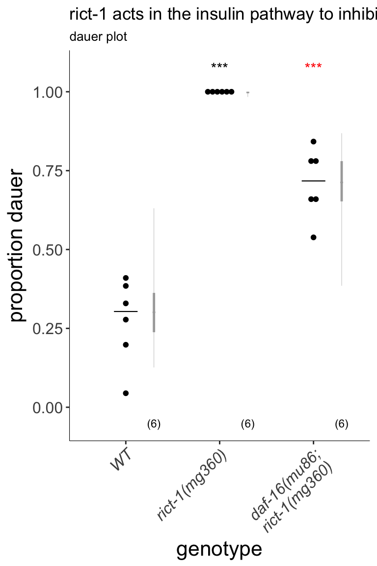
Figure S1E Mutations in rict-1 modulate dauer formation via downregulation of neuroendocrine signaling. daf-16 mutations partially suppress the dauer formation phenotype of rict-1 mutants. Dauers formed by animals of the indicated genotypes at 27°C. Each dot indicates the proportion of dauers formed in a single assay. Horizontal bar indicates median. Light gray thin and thick vertical bars at right indicate Bayesian 95% and 75% credible intervals, respectively. Numbers in parentheses below indicate the number of independent experiments with at least 26 animals each. *** - different from wild-type at P<0.001, *** - different from rict-1(mg360) at P<0.001 (ANOVA with Tukey-type multivariate-t post-hoc adjustments). P-values of differences in means relative to wild-type and corresponding mutant animals are indicated in black and red, respectively.
library(sjPlot)
sjt.lm(lm, depvar.labels = "proportion of dauers", show.se = TRUE, show.fstat = TRUE)
|
|
|
proportion of dauers
|
|
|
|
B
|
CI
|
std. Error
|
p
|
|
(Intercept)
|
|
0.27
|
0.19 – 0.36
|
0.04
|
<.001
|
|
genotype
|
|
rict-1(mg360)
|
|
0.73
|
0.60 – 0.85
|
0.06
|
<.001
|
|
rict-1;daf-16
|
|
0.44
|
0.31 – 0.56
|
0.06
|
<.001
|
|
Observations
|
|
18
|
|
R2 / adj. R2
|
|
.912 / .901
|
|
F-statistics
|
|
77.980***
|
knitr::kable(contrasts, caption="Pairwise comparisons from ANOVA (Tukey)")
Pairwise comparisons from ANOVA (Tukey)
| N2 - rict-1(mg360) |
-0.7259908 |
0.0585246 |
15 |
-12.404877 |
0.0000000 |
*** |
| N2 - rict-1;daf-16 |
-0.4360625 |
0.0585246 |
15 |
-7.450922 |
0.0000025 |
*** |
| rict-1(mg360) - rict-1;daf-16 |
0.2899283 |
0.0585246 |
15 |
4.953954 |
0.0004504 |
*** |
knitr::kable(mixed[,c(6,1:5)], caption = "Bayesian credible intervals")
Bayesian credible intervals
| N2 |
0.3009765 |
0.1261611 |
0.6307367 |
0.2378515 |
0.3625799 |
| rict-1(mg360) |
0.9979362 |
0.9835708 |
0.9998078 |
0.9956347 |
0.9989622 |
| rict-1;daf-16 |
0.7126570 |
0.3850782 |
0.8685749 |
0.6525277 |
0.7801805 |